Remote Sensing Lab 5

Goal and Background - This lab focused on analytic processes such as image enhancement, binary change detetion, image mosaic, band ratio, and spatial modeling. All of these within the context of Erdas Imagine 2013.

Methods and Results - The first skill we learned was image mosaics. I took two satellite images that over lap spatially both taken in May 1995. We first used the Mosaic Express tool (fig. 1) and then using the MosaicPro tool (fig. 2). The one made using the MosaicPro comes out better due to the use of Color Corrections which blended the two images more smoothly along the shared boundaries.

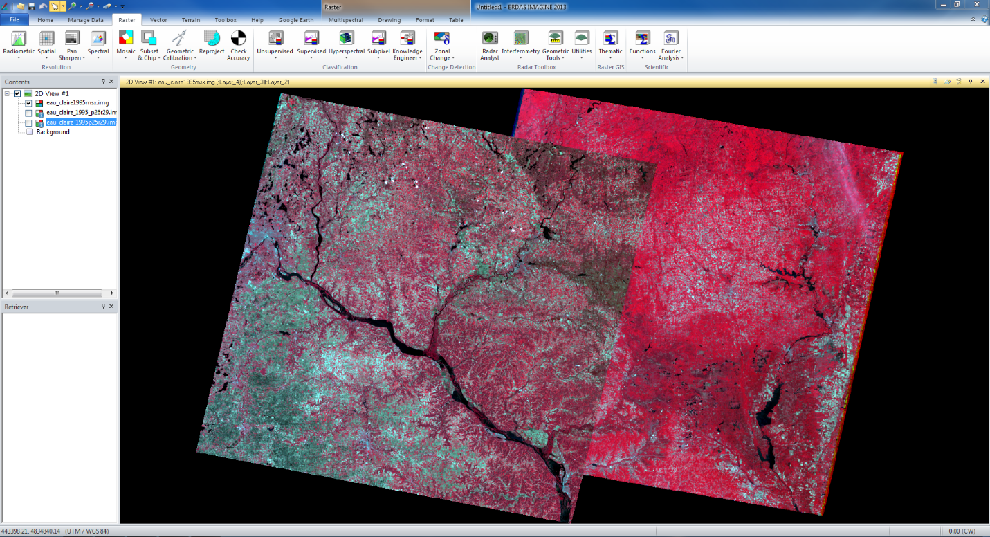fig. 1

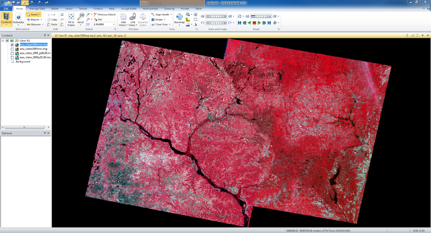fig. 2

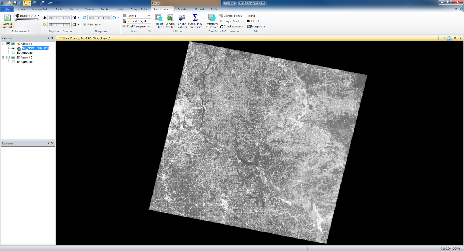
The second section deals with Band Ratios. We used the normalized difference vegetation index (NDVI) on an image of the Eau Claire area (fig. 3). It shows vegetation as the very white portions of the output image. The dark areas indicate rivers, roads, urban areas, and less healthy vegetation.

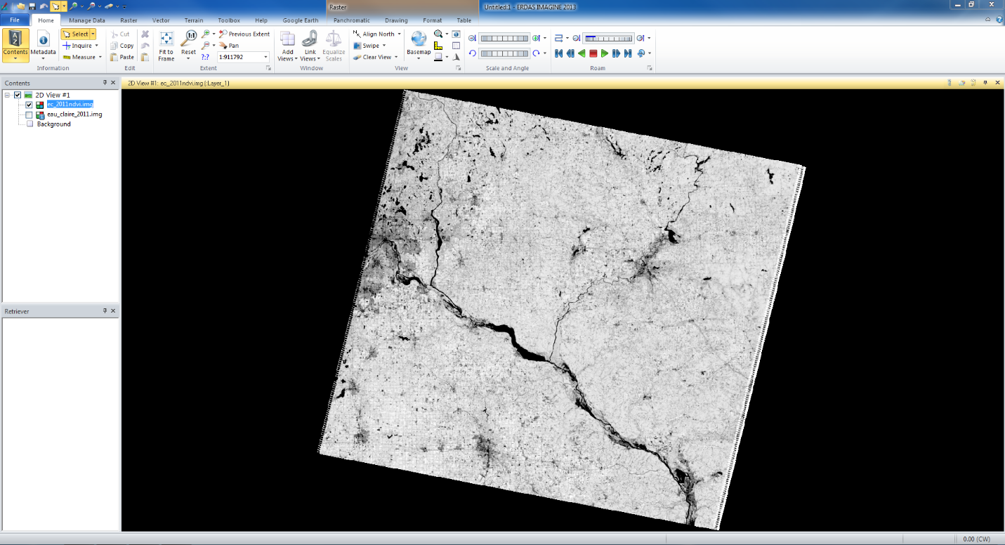fig. 3

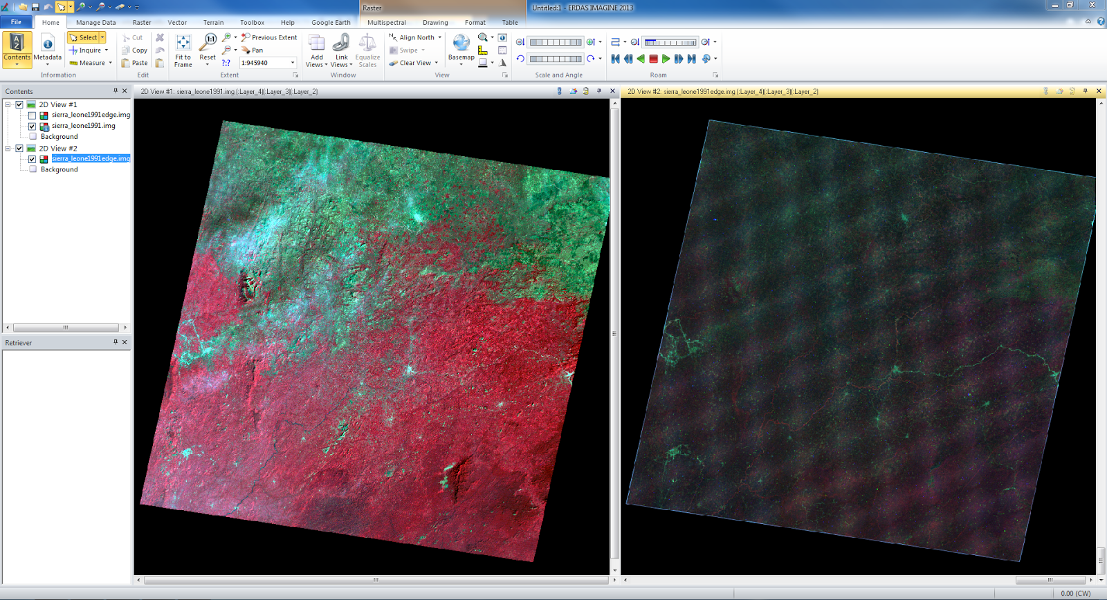
The next part introduced us to spatial image enhancement. The low frequency image from Sierra Leone on the left (fig. 4) shows how it is hard to see details when their is little contrast. The image on the right is the enhanced image and shows much more contrast. It is a very dark image, but we learn how to fix that in a later part.

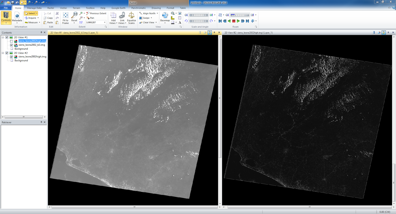fig. 4

We then performed a Laplacian convoultion filter on another image of Sierra Leone (fig. 5) which increases the contrast at discontinuities. It brings out features such as roads, cities and rivers.

fig. 5

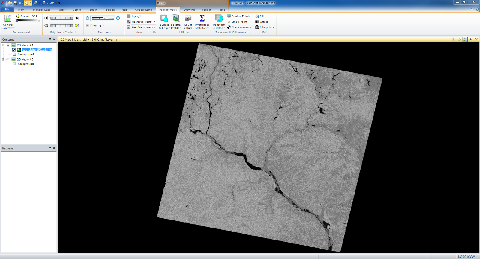
In the next section we practiced spectral enhancement. We performed minimum-maximum contrast stretch (fig. 6) on an image of Eau Claire that had a Gaussian histogram. On the second image of Eau Claire which was an NIR image we used a piecewise contrast stretch (fig. 7). We also performed a Histogram Equalization which spread a low frequency histogram across the whole range creating a high contrast image.

fig. 6

fig. 7

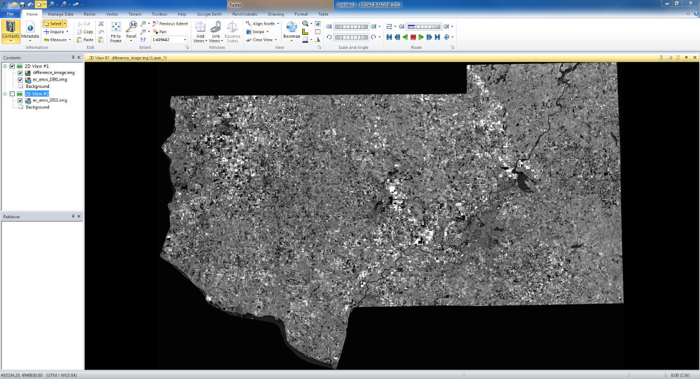
The final part dealt with binary change detection and image difference. We took an image of the Eau Claire region from 1991 and another of the same area from 2011 and we wanted to find the parts that changed in those 20 years. We first created a difference image (fig. 8) to show what pixels changed from 1991 to 2011.

fig. 8

 We then used the Model Maker tool to create a model that got rid of the pixels that stayed the same from 1991 to 2011 and created a difference image that only showed the areas that changed in the time period. I then opened ArcMap and overlaying the image of the changed area on top of a map of the region (fig. 9) showing the areas that changed in the region between 1991 and 2011 in red. It showed that the areas that changed were all agricultural lands.

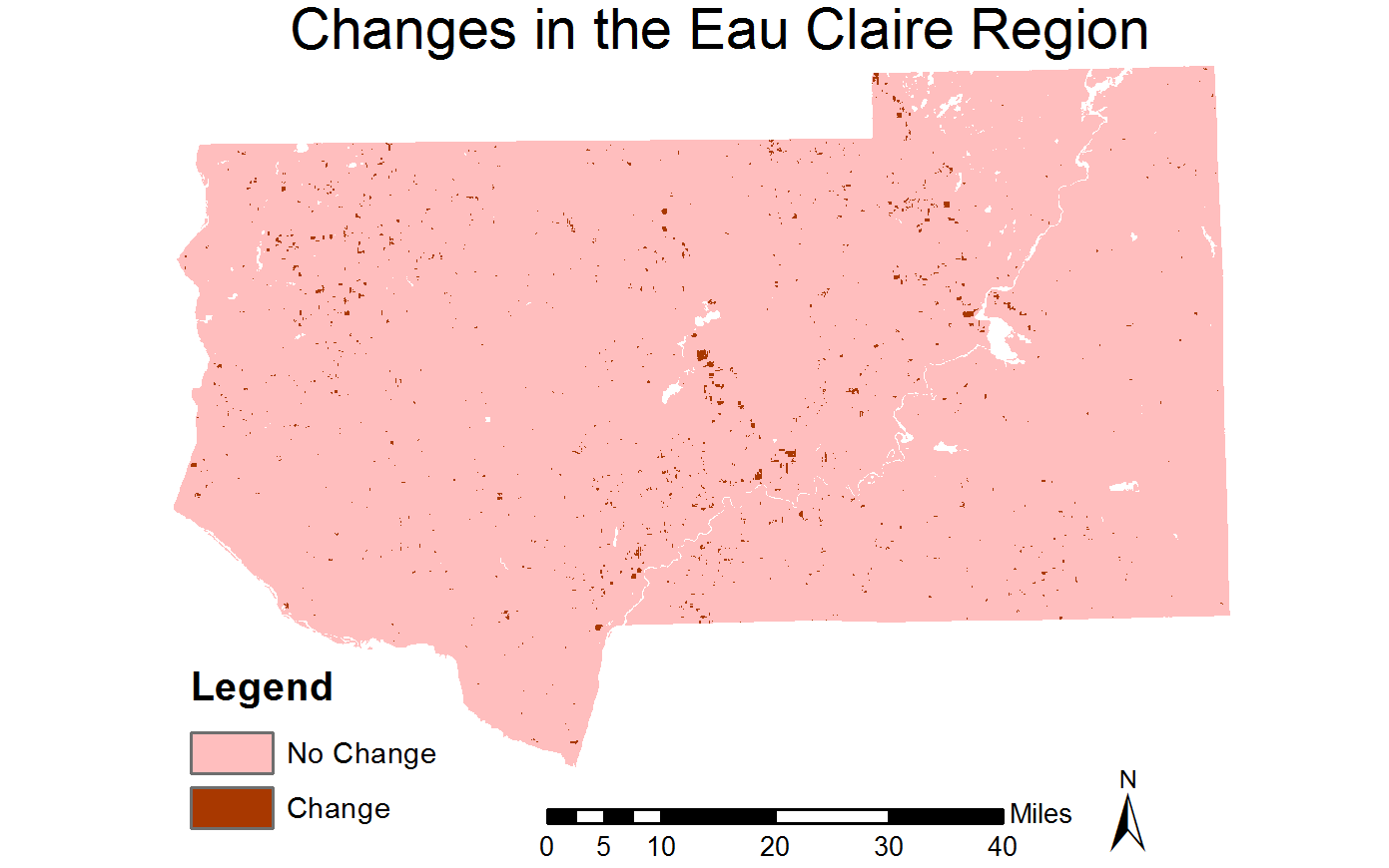fig. 9

Sources - All satellite images provided by Cyril Wilson.